With the development of the flow metering industry, plug-in electromagnetic flow meters are widely used in the measurement of large-diameter pipe flow because of their low cost, convenient installation and maintenance. Although the plug-in electromagnetic flowmeter measurement is a point measurement, a probe that is inserted into a pipe, that is, two electrodes on the sensor, collects signals and detects the information of the fluid in a certain area.

Nowadays, most people use the fluid dynamics (CFD) method to simulate the flow field, and the most widely used numerical solution is the finite volume method. The simulation software FLU-ENT used in this paper is based on this. Many people use the CFD method to perform plug-in electromagnetic flowmeter flow field simulation, often unable to determine its computational domain in the pipeline, leading to its signal simulation is difficult to achieve. In view of this situation, this paper uses FLUENT software to carry out three-dimensional numerical simulation of the flow field in the pipeline, and proposes the concept of signal range and the determination method.

1 Basic principles

1.1 Definition of signal range

According to the working principle of the plug-in electromagnetic flowmeter, the farther away from the electrode, the weaker the magnetic induction; when far away from a certain distance, the electromotive force generated by the fluid cutting magnetic induction line is weak to produce no fluid detection result. influences. Therefore, for the large-diameter pipeline, the flow signal that can be detected by the sensor electrode of the plug-in electromagnetic flowmeter is actually an electrical signal in a space area near the sensor probe in the pipeline to be measured, rather than covering the entire pipeline.

Therefore, a clear definition of the signal range is given in this paper. The signal action range refers to a certain spatial region near the electrode. The electromotive force generated by cutting the magnetic induction line in the conductive fluid in the region plays a decisive role in the flow detection result.

1.2 Definition of equivalent radius R

In the flow field, the stronger the signal, the easier it is to be received by the electrode. The size of the signal generated at each point in the field is related to the flow rate at that point, while the plug-in electromagnetic flowmeter changes the distribution of the flow field due to the insertion of the probe. Therefore, it can be seen that the electrodes are not equidistantly collecting effective signals around them, that is, the actual signal range is irregular. To facilitate the study, the equivalent signal range is defined by the following method. A spherical region VR with a radius R around the electrode makes its contribution to the signal with the actual signal range equivalent, ie satisfies equation (1).

(1)

In formula (1), Π is the actual overall area where the magnetic field of the fluid is cut by the fluid in the flow field. VR is the area where the electrode is the sphere center. The radius R is defined as the equivalent radius, Φ (x, y). z) is the signal that contributes to the unit volume of fluid in the flow space. As long as the equivalent radius R is determined, the effective signal range VR can be characterized.

1.3 Equivalent radius R research method

According to the calculation formula of volume flow, we can know:

QV=AU (2)

U in formula (2) refers to the average surface velocity of section A. The actual detected flow rate at the time of meter measurement should be the overall average flow velocity within the signal range. The conversion coefficient K of the meter can be obtained through standard device verification, and the overall average flow velocity within the signal range can be converted to the smallest pipe at the electrode location. The average flow velocity of the cross-section (abbreviated to the smallest cross section) to calculate the flow value. Therefore, in the simulation, the average flow velocity within the signal range can be used instead of the average velocity of the minimum cross section. Through this principle, the signal range can be solved and verified.

1.4 Equivalent Radius R Analysis Procedure

For the determination of the equivalent radius R, FLUENT software was used to simulate the large-diameter pipe inserted into the probe. The steps are as follows: 1 Obtain the relation between the radius r of different regions and the average flow velocity within the spherical region of the radius at a certain incoming flow velocity U; 2 Obtain the theoretical average flow velocity of the smallest cross section according to the continuity equation; 3 Use the interpolation method Determine the equivalent radius R of the signal range under the flow velocity; 4 Repeat the simulation experiment by changing the flow velocity.

2 How to determine the signal range

2.1 Determining the Calculation Domain

In order to ensure the quality of the grid, a cylindrical two-electrode probe with a wide range of structures and a simple structure is selected as a simulation object, and the calculation domain is shown in FIG. 1 . On the basis of ensuring the straight pipe sections before and after, set the water at normal temperature and pressure as the flowing medium, the inlet boundary condition is the speed inlet, and the outlet boundary condition is the pressure outlet. Select the standard k-ε model as the turbulence model, and its empirical constants C1ε, C2ε, C3ε takes 1.44, 1.92, and 0.09, respectively, and the turbulent kinetic energy and dissipation rate take 1.0 and 1.3, respectively.

According to the concept of signal range, as long as the probe can detect the flow signal, indicating that the flow at the location is within the scope of the magnetic field, the average speed in the calculation domain is:

(3)

In formula (3), Vr is the calculation area and u(x, y, z) is the speed function.

Figure 1 Plug-in electromagnetic flowmeter calculation domain

2.2 The Solution of the Theoretical Flow Rate of the Minimum Cross Section

The background of the research is plug-in electromagnetic flowmeters for measuring the flow of large-diameter pipes. Therefore, the pipe model used is a large-diameter pipe with the following dimensions: the pipe diameter is 400mm, the probe radius is 32mm, the electrode radius is 5mm, and the probe The insertion depth is 120mm.

From the continuity equation can be obtained:

(4)

In equation (4), U is the actual flow velocity, and A1 is the cross-sectional area of ​​the pipeline. For the minimum cross-sectional theoretical flow rate, A2 is the minimum cross-sectional area.

Using GAMBIT software to establish the model, we can directly get A2=117961.70mm2. Take the 6 velocity point with a flow velocity in the range of 0.5 to 10 m/s. Then, according to equation (4), find the theoretical flow rate at the minimum cross section at different flow velocity. .

2.3 The relation between the average velocity in the calculation domain and the radius of the calculation domain

Taking the radius of the calculation domain in the range of 10 to 80 mm, the models were established by GAMBIT software, and then simulated by FLUENT software. The volume-weighted average velocity corresponding to different radiuses in the computational domain was obtained, as shown in Table 1.

Table 1 Average Flow Velocities at Different Computational Domain Radiuses

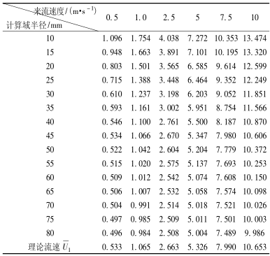
From the data in Table 1, it can be seen that as the radius of the calculation domain increases, the average flow velocity in the calculation domain gradually decreases. This is because when the radius of the computational domain is small, the turbulent flow near the probe is relatively violent, resulting in an excessively large mean flow velocity in this region. When the radius of the computational domain is large, the fluid flow in the outermost region is weakened. Those areas do not play a decisive role in the signal, resulting in an average flow rate that is too small. It also indicates the existence of an effective signal range.

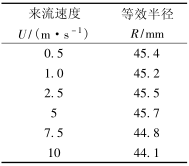
In order to obtain equivalent radii at different flow velocities, MATLAB was used to interpolate the corresponding theoretical flow rates for each set of data, and the data shown in Table 2 was obtained.

Table 2 Equivalent Radius at Different Incoming Velocities

2.4 Determine R

From Table 2, it can be seen that although the flow velocity is different, the difference between the corresponding equivalent radii is not very large, and it can even be said to be very close. Calculate the relationship between the radius of the calculation domain and the velocity curve at any different flow velocity and compare them, as shown in Figure 2. From the figure, it can be seen that although the flow rates are different, the radius of the calculation domain is the same, that is, the horizontal axis is consistent, and the shapes of the curves are very similar. Therefore, it can be considered that the size of the equivalent radius is independent of the flow velocity.

From the above analysis, it can be concluded that the equivalent radius R is a fixed value, that is, the range of equivalent signals obtained is a fixed value. That is to say, in the case that the magnetic circuit system of the flow sensor does not change, the effective signal range does not change with the change of the flow speed.

In order to reduce the calculation error and improve the confidence of the data, the average of each equivalent radius in Table 3 is obtained as R, that is:

Table 3 Comparison of Instrument Value and Simulation Value

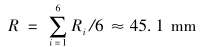(5)

Fig. 2 Comparison of signal range at any two flow rates

FNH Air Cooling Condenser

China Evaporator And Condenser,Chiller Condenser manufacturers, welcome Refrigeration Condensing Unit,Evaporative Cooled Condenser purchasers from worldwide to visit our site.

Fin type air cooled condenser is one of high efficient condensing heat exchangers designed for refrigeration compressor condensing units and multi-compressor units. We have H type, V type and W type with different width, length and different air direction meet your different needs.Up blow air direction and lateral blow direction can insure best fittings. Different fan quantity can insure condensing pressure adjusting. Fin type condensers equip with axial fan can reduce motor noise refrigeration capacity covers form 6KW to 227KW fitting diiferent kind of refrigerant such as R134a, R404Aa,R507a,R407C.

Evaporator And Condenser,Chiller Condenser,Refrigeration Condensing Unit,Evaporative Cooled Condenser

Zhejiang Diya Refrigeration Equipment Co.,LTD. , https://www.diyarefrigeration.com